bmi_dbseabed package provides a set of functions that allow downloading of the datasets from dbSEABED, a system for marine substrates datasets across the globe. This system uses very large amounts of diverse observational data and applies math methods to integrate/harmonize those and produces gridded data on the major properties of the seabed. The scope is the global ocean and across all depth zones.
The current page serves only the data for the Gulf of Mexico region (Bounding box: west=-98, south=18, east=-80, north=31). An overview of the entire collection of data is available at this webpage. Please note that the data will be updated from time to time, approximately annually.
bmi_dbseabed package includes a Basic Model Interface (BMI), which converts the bmi_dbseabed dataset into a reusable, plug-and-play data component (pymt_dbseabed) for the PyMT modeling framework developed by Community Surface Dynamics Modeling System (CSDMS).
Installation
Stable Release
The bmi_dbseabed package and its dependencies can be installed with either pip or conda,
pip install bmi_dbseabed
conda install -c conda-forge bmi_dbseabed
From Source
After downloading the source code, run the following command from top-level folder to install bmi_dbseabed.
pip install -e .
Citation
Please include the following references when citing this software package:
Gan, T., Tucker, G.E., Hutton, E.W.H., Piper, M.D., Overeem, I., Kettner, A.J., Campforts, B., Moriarty, J.M., Undzis, B., Pierce, E., McCready, L., 2024: CSDMS Data Components: data–model integration tools for Earth surface processes modeling. Geosci. Model Dev., 17, 2165–2185. https://doi.org/10.5194/gmd-17-2165-2024
Gan, T., & Jenkins, C. (2025). CSDMS dbSEABED Data Component. Zenodo. https://doi.org/10.5281/zenodo.15021967
Quick Start
Below shows how to use two methods to download the datasets.
You can learn more details from the tutorial notebook. To run this notebook, please go to the CSDMS EKT Lab and follow the instruction in the “Lab notes” section.
Example 1: use DbSeabed class to download data (Recommended method)
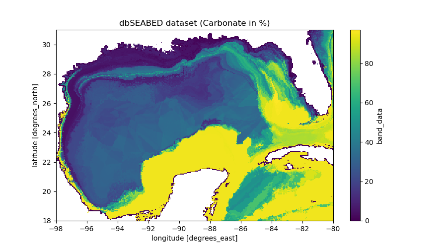
In this example, it downloads the surficial seafloor carbonate fraction (var_name=”carbonate”). To learn all supported data variables, please check the “var_name” from the Parameter settings.
import matplotlib.pyplot as plt
from bmi_dbseabed import DbSeabed

# get data from dbSEABED
dbseabed = DbSeabed()
data = dbseabed.get_data(
    var_name="carbonate",
    west=-98,
    south=18,
    east=-80,
    north=31,
    output="download.tif",
)

# show metadata
for key, value in dbseabed.metadata.items():
    print(f"{key}: {value}")


# plot data
data.plot(figsize=(9, 5))
plt.title("dbSEABED dataset (Carbonate in %)")
Example 2: use BmiDbSeabed class to download data (Demonstration of how to use BMI).
import matplotlib.pyplot as plt
import numpy as np

from bmi_dbseabed import BmiDbSeabed


# initiate a data component
data_comp = BmiDbSeabed()
data_comp.initialize("config_file.yaml")

# get variable info
var_name = data_comp.get_output_var_names()[0]
var_unit = data_comp.get_var_units(var_name)
var_location = data_comp.get_var_location(var_name)
var_type = data_comp.get_var_type(var_name)
var_grid = data_comp.get_var_grid(var_name)

print(f"{var_name=} \n{var_unit=} \n{var_location=} \n{var_type=} \n{var_grid=}")

# get variable grid info
grid_rank = data_comp.get_grid_rank(var_grid)

grid_size = data_comp.get_grid_size(var_grid)

grid_shape = np.empty(grid_rank, int)
data_comp.get_grid_shape(var_grid, grid_shape)

grid_spacing = np.empty(grid_rank)
data_comp.get_grid_spacing(var_grid, grid_spacing)

grid_origin = np.empty(grid_rank)
data_comp.get_grid_origin(var_grid, grid_origin)

print(f"{grid_rank=} \n{grid_size=} \n{grid_shape=} \n{grid_spacing=} \n{grid_origin=}")

# get variable data
data = np.empty(grid_size, var_type)
data_comp.get_value(var_name, data)
data_2D = data.reshape(grid_shape)

# get X, Y extent for plot
min_y, min_x = grid_origin
max_y = min_y + grid_spacing[0] * (grid_shape[0] - 1)
max_x = min_x + grid_spacing[1] * (grid_shape[1] - 1)
dy = grid_spacing[0] / 2
dx = grid_spacing[1] / 2
extent = [min_x - dx, max_x + dx, min_y - dy, max_y + dy]

# plot data
fig, ax = plt.subplots(1, 1, figsize=(9, 5))
im = ax.imshow(data_2D, extent=extent)
fig.colorbar(im)
plt.xlabel("X")
plt.ylabel("Y")
plt.title("dbSEABED dataset (Carbonate in %)")

# finalize data component
data_comp.finalize()
Parameter settings
“get_data()” method includes multiple parameters for data download. Details for each parameter are listed below.
var_name: The identifier of each dataset provided by dbSEABED. The identifiers and the corresponding BMI standard names are shown below (var_name: BMI standard name). The “data_services” attribute of an instance will show more information for each identifier such as url link and variable unit for each dataset. To learn more information about these supported datasets, please check this webpage.
carbonate: surficial_seafloor_carbonate__fraction
carbonate_totlsu: surficial_seafloor_carbonate__fraction_uncertainty
grainsize: surficial_seafloor_sediment__grain-size
grainsize_totlsu: surficial_seafloor_sediment__grain-size_uncertainty
gravel: surficial_seafloor_sediment_gravel__fraction
gravel_totlsu: surficial_seafloor_sediment_gravel__fraction_uncertainty
mud: surficial_seafloor_sediment_mud__fraction
mud_totlsu: surficial_seafloor_sediment_mud__fraction_uncertainty
organic_carbon: surficial_seafloor_sediment_organic-carbon__fraction
organic_carbon_totlsu: surficial_seafloor_sediment_organic-carbon__fraction_uncertainty
rock: surficial_seafloor_rock~exposed__fraction
rock_totlsu: surficial_seafloor_rock~exposed__fraction_uncertainty
sand: surficial_seafloor_sediment_sand__fraction
sand_totlsu: surficial_seafloor_sediment_sand__fraction_uncertainty
west, south, east, north: The bounding box (extent) values for the downloaded data. These values should be based on the coordinate system (EPSG: 4326) of the datasets from dbSEABED. The west and south values are for the lower left corner of the grid extent. The east and north values are for the upper right corner of the grid extent.
output: The file path of the GeoTiff file to store the downloaded data with “.tif” file extension.
local_file: Indicate whether to make it priority to get the data by loading a local file that matches with the output file path. Default value is set as False, which means the function will directly download the data from dbSEABED system. If value is set as True, the function will first try to open a local file that matches with the output file path. And if the local file doesn’t exist, it will then download data from dbSEABED.